
Object detection with synthetic data
- Neurolabs Wix
- Dec 7, 2020
- 7 min read
Reduce the domain gap with domain randomization
In this post, we’ll explore how we can improve the accuracy of object detection models that have been trained solely on synthetic data.
Why machine learning? Why simulate data?
Since the resurgence of deep learning for computer vision through AlexNet in 2012, we have seen improvement after improvement — deeper networks, new architectures, more availability in data — with records being broken for accuracy and prediction speed year after year.
Object detection, a subset of computer vision, solves the problem of identifying and localising classes in an image. Image classification answers the question “what is this image of”; image localisation answers “where are all the objects in this image”; and object detection combines the two to find the objects in the scene and identify them.
The advances in object detection have made state-of-the-art results accurate and practical for commercial use, but it is still being held back by quick access to large amounts of training data. Furthermore, even if you have assembled the perfect data set, imagine that the conditions of your environment change (for example outdoors instead of indoors): the data gathering process starts anew.
Advances in computer graphics have made special effects, animated movies and video games almost indistinguishable from real life. These techniques allow you to conceptually build complex virtual worlds with a limitless range of possibilities for the environment.
At Neurolabs, we believe that synthetic data holds the key for better object detection models, and it is our vision to help others to generate their own bespoke data set or machine learning model.
A small word on other approaches to synthetic data generation. Synthetic data can also be done by discovering the underlying distribution of your data: once you would have this, you could sample infinitely for new data points. This is however a chicken-and-egg type problem: if you could perfectly find this distribution, your object detection problem would be solved and wouldn’t have to generate more data, synthetic or otherwise. Naturally, such techniques rely heavily on approximation, which may gloss over the edge cases and negate exactly the reason for which simulation was deployed in the first place. The example to consider is the following: if you only approximate car positions on the road, you would miss the rare cases where a car is flipped.
Problems with domain transfer
A pressing problem in machine learning is that of domain transfer: train a model on a specific domain, and then deploy it on another. A domain could be a slightly different environment, or a slight variation in the distance of the camera, or data that was simulated into existence.
The suggested solutions to ‘bridging the domain gap’ can be grouped into the following: domain adaptation, domain generalisation and domain randomisation. We will focus on domain randomisation for the remainder of the article.
Domain randomisation tries to solve the domain transfer problem by increasing the variation of the training data, simply by applying randomness to an object’s properties and the environment. Doing so should in effect broaden the model’s understanding of the intrinsic features that define the object, instead of focusing only on the incarnations appearing in the data. An example: a banana that’s twice as large, half as curved, a slightly different hue, covered with aging spots, is still a banana.
Neurolabs’ synthetic data engine
Neurolabs has built a synthetic data engine that’s capable of producing data at scale. We achieve this through an architecture that first creates a large amount of render tasks and secondly executes these rendering tasks in parallel — following a similar mindset to the serial and parallel split in Amdahl’s Law.
Render task definition — here we generate a large number of tasks with specific details of what objects will be rendered, in what environment, and in what configuration. Domain randomisation is performed at this step.
Rendering — our rendering is heavily parallelised, with each process/instance assigned a single task. Rendering involves taking a configuration file, along with a list of 3D assets, and then using a graphics engine to produce a set of images. The graphics engine we currently use is Blender, however, it is simple to exchange. The graphics engine must load the object files, set positions as specified in the configuration file, render the image, and determine the screen-space bounding box of the object.
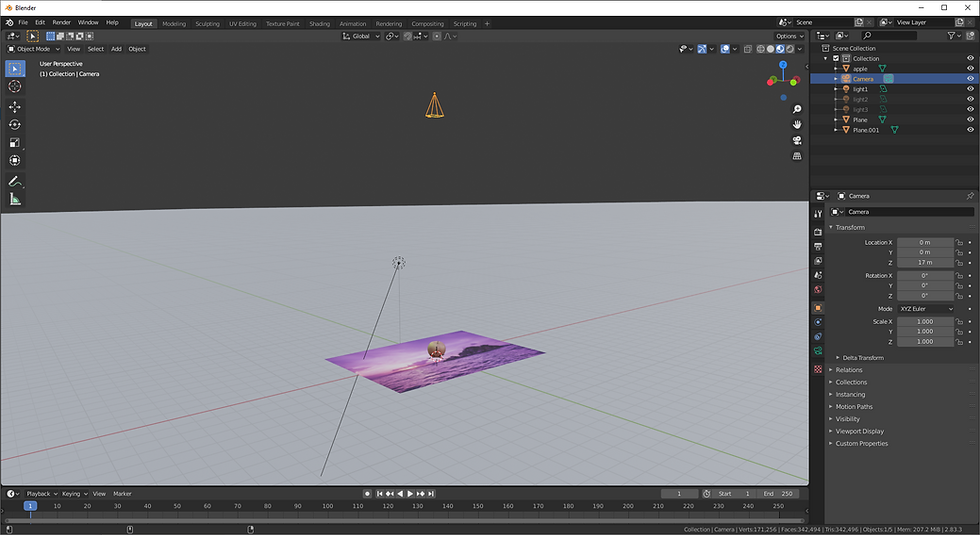
Figure 1 — a basic scene in Blender. Image by author.
Experiment
In order to determine how various object properties contribute to a better model under domain randomisation, we created a variety of data sets. We started with the first data set applying domain randomisation on all properties, and then removed randomisation of a single property in every subsequent data set.
Properties:
Scale — can vary between 1x and 2x the original size.
Rotation — can be any that are part of the natural rotations (e.g. bottles wouldn’t stand on their head).
Hue-Saturation-Value — changed the base colour of the object slightly.
Light position/number — change the number of lights and their position. Maximum luminosity is capped.
Light colour — change the colour of each of the lights.
The two additional properties that we did not remove randomisation from are:
Location — x, y position of the object, bounded by the cameras viewport.
Background — a variety of 50 images, randomly chosen per render task.

Figure 2 — HSV randomisation. Image by author.
Objects & classes
We used 6 classes: apples, bananas, broccoli, bread bun, croissant, orange.
For the real data set, we purchased the items from the local supermarket and annotated images.

Figure 3 — images from the real data set. Image by author.
For the synthetic data, we need 3D models of all the classes. We ensured that we have at least 2 different models per class. We used a combination of free assets from online marketplaces, or used RealityCapture to obtain the model using photogrammetry.

Figure 4–3D models rendered in Blender without lighting. Image by author.
Object detection framework
We used Detectron2 as the machine learning framework. Detectron2 has out-of-the-box support for Faster R-CNN, which usually ranks higher in terms of accuracy at the expense of performance compared to single step detectors. All of the experiments used transfer learning: we fine-tuned the pre-trained model from the model zoo with our data sets. The Faster R-CNN model’s backbone was ResNet-50 and used Feature-Pyramid Networks.
Runs
All of our experiments used Stochastic Gradient Descent with momentum as the optimiser and a learning rate of 0.00125, ran for 5 epochs (2000 iterations with 2 images per batch and 800 images), and ran a validation job twice per epoch using an evaluator that produces the same statistics as used for the COCO data set challenge. The evaluation data set had the same domain randomisation settings as the training data; only the test data set stayed constant across the runs. We ran the experiments on a single machine with an Nvidia GeForce RTX 2060 GPU; training and validation took around 30 minutes in total for each case.
Data set “none”: no randomisation.
Data set “r”: randomisation on rotation.
Data set “r-s”: randomisation on rotation and scale.
Data set “r-s-c”: randomisation on rotation, scale and hue-saturation-value.
Data set “r-s-c-lp”: randomisation on rotation, scale, hue-saturation-value and light position/count.
Data set “r-s-c-lp-lc”: randomisation on rotation, scale, hue-saturation-value, light position/count and light colour.
For each data set, 1000 images were generated and split, with 800 assigned to training, and 200 for validation. We generated the synthetic images locally with 6 processes, taking a total of 16 minutes. We consider this a true syn2real experiment, as no real data were used during the training nor validation phases.


Figure 5 — images from the synthetic data set. Image by author.
Here are the figures for the loss vs iteration. Keep in mind that these numbers are with respect to synthetic data only.

Figure 6 — total training/validation loss vs iteration. Image by author.
Here is the figure for the model’s ability to learn on synthetic data.

Figure 7 — mAP 50 during training vs iteration. Image by author.
Results
Here are the results for all of the data sets. The metrics are the commonly used mean average precision (mAP) with intersection-over-union (IoU) averaged over 10 thresholds (i.e. 0.5, 0.55, …, 0.95), mAP with IoU of 0.5, and mAP with IoU of 0.75.

Figure 8 — bar chart of test metrics. Image by author.
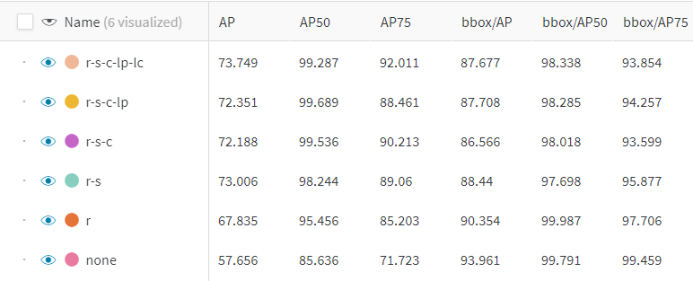
Figure 9 — table of results. AP are test results, bbox/AP are validation results. Image by author.
The results show that rotation and scale have the largest impact on helping the model generalise to the test domain. The various other properties help in achieving a more accurate overall detector, yet to a smaller degree. It is interesting to note that an increase in accuracy in one metric, doesn’t always translate to an increase in another.
Further results
Here are the results of the data set with domain randomisation for all properties compared with real and combined (800 synthetic and 100 real).

Figure 10 — bar chart of test metrics. Image by author.
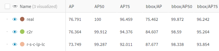
Figure 11 — table of results. AP are test results, bbox/AP are from validation. Image by author.
Training on real data yielded the best results, followed closely by combined (c2r), and finally the synthetic-only. The real data set had a lower evaluation mAP50-95, yet a higher mAP50 and mAP75 compared with the synthetic data sets, suggesting that the distribution of the synthetic data was not as varied per-class but had stronger inter-class similarities.
Conclusion
Domain randomisation has a significant impact on creating an object detector with better accuracy. All the properties that were subject to the randomisation had a positive impact on at least one of the metrics. Training on real data shows that the complexity in the synthetic domain needs to be further increased.
With regards to training: even though the typical number of epochs needed with transfer learning is substantially lower, the training and evaluation loss were still decreasing, meaning further training would be beneficial. The number of epochs and amount of synthetic training data was arbitrarily limited by the amount of time dedicated to training; we can use multi-GPU AWS EC2 instances to allay that concern.
While these preliminary findings show that real data yield the highest accuracy, synthetic data produced results that may be considered good-enough depending on the use-case. Considering that synthetic data does not require labelling any images, there is a clear incentive to use it for object detection, if only as a temporary solution before enough real data have been acquired.
We are currently exploring many other parameters on which to performance randomisation to catch-up to and overtake the real data accuracy. Furthermore, domain randomisation is only one of the ways that we can ‘bridge the domain gap’, and we look forward to sharing results for smart parameter search with you in the future.
Finally, we are making this data freely available to the public. Please find the synthetic data here, the real data here, and a demo page here.
Written by Markus Schläfli, Head of Simulation at Neurolabs
At Neurolabs, we believe that the lack of widespread adoption of machine learning is due to a lack of data. We use computer graphics, much like the special effects or video game industry, to produce realistic images at scale. In 5 minutes, you can have 10,000 images tailored for your problem. But we don’t stop there — we kick-start the machine learning training, and allow any industry to implement ready-made Computer Vision algorithms without an army of human annotators.


Comments